
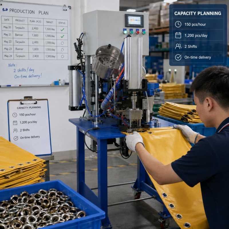
You do not buy production capacity in eyelets per minute. You sell curtains, banners, shoes, bags, tags, or other finished products—and each one consumes a different number of eyelet settings. That is why a machine speed printed in a catalogue cannot answer the question you actually have: how many automatic eyelet machines will cover your daily orders without turning every busy day into a recovery plan?
The calculation becomes manageable when you move in one direction: finished items, then required good eyelet settings, then usable production minutes, then cycles per minute, and finally machines required. This guide gives you that method. It is a demand-based sizing calculation for an automatic-machine cluster, not another argument about when you should upgrade.
Quick answer: calculate the good eyelet settings your order mix needs, divide that load by the good settings one machine can deliver in the same scheduled time, and round the result up. Use a representative production trial—not an empty-cycle maximum—to establish the machine rate.
Why Brochure Speed Is Not Your Capacity?
A quoted 40 cycles per minute usually describes a machine under defined conditions. Your shift includes breaks, product changes, feeder refills, first-piece checks, minor stops, cleaning, rejected settings, and material handling. Some products also limit how quickly the operator can present the next workpiece, even when the press itself can cycle faster.
The unit can be misleading too. One cycle may make one setting. A synchronized double-head machine may make two settings per cycle, but only when the two eyelet positions match the head spacing and both heads are used. A finished item may need two eyelets, six eyelets, or a mixed pattern. Capacity planning fails when cycles, settings, and finished items are treated as the same thing.
Before you use the calculator, confirm what happens inside one cycle in How Automatic Eyelet Machine Works. Feeding, punching, setting, inspection, and operator handling can each become the pace-limiting step.
The Inputs You Need
Collect these inputs for the same planning period—normally one day or one shift. Do not mix weekly demand with daily minutes.
| Symbol | Input | How you define it |
| D | Finished items required | Sum each SKU’s order quantity for the period. |
| E | Eyelet settings per item | Use each SKU’s actual count; use a weighted average only for a quick estimate. |
| P | Peak-demand factor | Peak demand divided by average demand, such as 1.15 for a 15% peak. |
| M | Net scheduled minutes per machine | Shift minutes minus breaks, planned changeovers, cleaning, and planned checks. |
| C | Validated cycles per minute | A sustained rate on your real material and hardware, after warm-up. |
| H | Good settings per cycle | Usually 1 for a single head; up to 2 for a synchronized double-head job. |
| A | Availability | Run time divided by planned production time. |
| R | Performance | Actual running speed divided by the validated ideal speed. |
| Q | Quality rate | Good settings divided by total settings attempted. |
| U | Planning utilization | Optional scheduling guardrail, often below 1.00, kept separate from physical losses. |
| N | Machines required | The result, always rounded up to a whole machine. |
Choose One Loss Method—Do Not Combine Both
You can calculate usable output from observed good production or from separate loss factors. Both methods work. The mistake is using an observed rate that already includes stops and rejects, then multiplying it by availability and quality again. That makes the estimate artificially low.
Method A: observed good output
Use this method when you have a timed trial or production history. Divide accepted settings by the full scheduled minutes in the observation window. Keep normal minor stops, misfeeds, and rejects in the count.
Observed good settings per scheduled minute = accepted settings ÷ scheduled minutes
Good capacity per machine = M × observed good settings per scheduled minute × U
This is usually your safest planning method because it measures what the whole station delivered, not what the press did during its cleanest ten seconds.
Method B: component loss model
Use this method when you know the validated cycle rate and can defend separate availability, performance, and quality assumptions.
Good capacity per machine = M × C × H × A × R × Q × U
Availability, performance, and quality mirror the standard OEE structure. Availability covers stopped time, performance covers slow running and small stops, and quality covers rejected settings. Your planning utilization U is different: it is an intentional scheduling guardrail for variability or unscheduled work. If your peak factor and loss history already provide enough protection, set U to 1.00 rather than adding an unexplained second cushion.
The Capacity Planning Calculator
Step 1: convert daily orders into good eyelet settings

For one product:
Good settings required = finished items ordered × eyelet settings per item
For a mixed order book:
Total good settings required = Σ (SKU quantity × eyelet settings per SKU)
Calculate each SKU before you add the totals. A simple average eyelet count can understate demand when your high-volume SKU also carries the highest number of eyelets.
Step 2: apply the demand scenario
Planned good settings = total good settings required × peak-demand factor
Use a peak factor from order history, not a comfortable guess. If your 90th-percentile day is 18% above an average day, use 1.18 for that service scenario. You can run base, peak, and launch/rush cases side by side instead of hiding uncertainty in one oversized factor.
Step 3: calculate net scheduled minutes
Net scheduled minutes = total shift minutes − breaks − planned changeovers − planned cleaning/checks
Subtract planned losses here. Leave unplanned downtime in availability or in your observed good rate. If you subtract the same loss from minutes and from availability, you count it twice.
Step 4: calculate capacity per machine
Observed-rate path: machine capacity = M × observed good settings/min × U
Component path: machine capacity = M × C × H × A × R × Q × U
Step 5: calculate machines required
N = ROUND UP (planned good settings ÷ good capacity per machine)
Always round up. A result of 2.05 does not mean two machines with a little effort. It means two machines are short under the assumptions you chose. The calculation does not decide what you buy; it exposes the load that your schedule must cover.
Step 6: convert the result back to required cycles per minute
Once you choose a cluster size, calculate the sustained cycle rate each machine must support. This lets you test a candidate configuration against real trial data.
Required C = planned good settings ÷ (N × M × H × A × R × Q × U)
If you use Method A, the equivalent check is simpler: required observed good settings per scheduled minute = planned good settings ÷ (N × M × U).
Worked Example: Sizing an Automatic-Machine Cluster
Suppose you need to plan one production day for three products. You run two 480-minute shifts. After breaks, two changeovers, cleaning, and first-piece checks, each machine has 810 net scheduled minutes.
| SKU | Items/day | Settings/item | Good settings/day |
| A | 8,000 | 2 | 16,000 |
| B | 5,000 | 4 | 20,000 |
| C | 2,000 | 6 | 12,000 |
| Total | 15,000 | — | 48,000 |
Your peak-day factor is 1.15, so planned good settings are 48,000 × 1.15 = 55,200. Your validated machine rate is 36 cycles per minute with one setting per cycle. From representative runs, availability is 0.87, performance is 0.90, and quality is 0.985. You also choose a planning utilization of 0.85 because the cluster must absorb normal scheduling variation.
Good capacity per machine = 810 × 36 × 1 × 0.87 × 0.90 × 0.985 × 0.85
Good capacity per machine = 19,116 settings/day
Machines required = ROUND UP (55,200 ÷ 19,116) = 3 machines
Now check the required cycle rate for a three-machine cluster: 55,200 ÷ (3 × 810 × 1 × 0.87 × 0.90 × 0.985 × 0.85) = 34.7 cycles per minute per machine. A machine validated at 36 cycles per minute clears the scenario, but with little speed margin inside the assumptions.
This conclusion is more useful than saying that one machine can run at a high maximum speed. It connects your product mix, schedule, production losses, and service target in one auditable line.
How to Handle Mixed Products and Changeovers?
A mixed factory rarely runs one eyelet, one washer, and one material all day. Product mix changes both demand and usable time. Treat it explicitly.
- Calculate settings by SKU. Multiply each order quantity by its own eyelet count before summing.
- Group families that share a feeder, raceway, die set, material presentation, and quality standard.
- Subtract planned changeover time from scheduled minutes. Include first-piece approval and trial pieces if they consume the machine.
- Use the slowest validated rate for a family only when it is genuinely representative. Otherwise calculate load in minutes by SKU: required settings ÷ validated good settings per minute, then add setup minutes.
- Check the calendar, not just the total. Three machines may have enough daily capacity but still miss an early dispatch if the same tooling is needed at the same time.
For a high-mix schedule, the load-in-minutes method is often clearer: total required machine minutes = Σ (SKU good settings ÷ SKU validated good rate) + total changeover minutes. Compare that load with the available machine-minutes in your cluster.
Cluster Constraints the Formula Cannot See
The arithmetic assumes each machine can use its calculated minutes. Your floor may impose a harder limit. Review these constraints before you accept the result.
- Operator coverage: one operator may supervise several stable feeders, but manual presentation, inspection, material lifting, or frequent replenishment can reduce that ratio.
- Feeder and hardware consistency: burrs, flange variation, coating residue, and mixed lots can turn a fast press into a stop-start station.
- Shared tooling: one spare die set, gauge, or technician can become the true constraint during changeovers or faults.
- Utilities: compressed-air pressure, electrical supply, extraction, and floor layout must support simultaneous operation, not one-machine trials.
- Upstream and downstream flow: cutting, marking, inspection, packing, or material transport can starve or block the cluster.
- Double-head geometry: count two settings per cycle only for products that can present both positions at the required spacing and orientation.
If feeding instability is a recurring loss, use the checks in How to Improve Feeding Stability in Automatic Eyelet and Snap Button Systems before you assume the answer is simply a higher cycle rate.
Validate the Rate on Good Output
Your calculator is only as reliable as C, A, R, and Q—or the observed good rate that replaces them. Validate those numbers on your actual eyelets, washers, materials, thickness range, and operator method. Run long enough for the feeder, dies, drive, sensors, and material handling to reach normal working conditions.
If the machine cycles consistently but the station rate is lower, review operator handling and workstation ergonomics because material support, reach distance, pedal position, inspection, and removal can become the limiting steps.
During the trial, record:
- scheduled start and finish time;
- total cycles and accepted settings;
- rejects, jams, misfeeds, missing washers, and manual interventions;
- downtime by reason;
- changeover and first-piece approval time;
- the exact eyelet, washer, material, thickness, tooling, and operator method.
Use accepted parts, not empty cycles. The Eyelet Machine Acceptance Test Checklist explains what to record during a sustained test. Before testing, use What Samples to Send Before an Eyelet Machine Trial so the trial represents your actual production range.
A Practical Data Collection Routine
If you do not yet have trustworthy loss factors, start with five representative production days. For each machine and product family, record scheduled minutes, run minutes, total settings, good settings, and changeover minutes. Then calculate:
- Availability = run minutes ÷ planned production minutes
- Performance = total settings ÷ (run minutes × validated ideal settings per minute)
- Quality = good settings ÷ total settings
- Observed good rate = good settings ÷ scheduled minutes
Use the median day for a typical scenario and a lower-percentile day for a conservative scenario. Keep unusual events visible rather than deleting them without explanation. A supplier delay or power failure may not belong in a machine-performance factor, but repeated feeder stops certainly do.
Maintain the assumptions that affect stable output with the Eyelet Punching Machine Maintenance Checklist for Stable Daily Output. Capacity is a maintained condition, not a permanent catalogue property.
Common Capacity Planning Mistakes
| Mistake | Correction |
| Using finished items as cycles | One product can consume several settings. Convert the order mix first. |
| Using maximum speed as sustained speed | Validate on the real product after warm-up and count accepted output. |
| Double-counting losses | Do not apply availability and quality to an observed rate that already contains them. |
| Counting two heads on every job | Use H = 2 only when both heads produce acceptable settings in each cycle. |
| Ignoring changeovers | Subtract planned setup time or add setup minutes to the load. |
| Sizing to the average only | Run a peak scenario based on order history and service commitments. |
| Assuming every machine is independent | Check shared operators, tooling, utilities, material flow, and inspection. |
| Rounding down | A fraction above a whole number is an uncovered load, not spare capacity. |
FAQ
What is a realistic eyelet machine cycles-per-minute figure?
It is the sustained rate validated on your eyelet, washer, material, tooling, and handling method. Published machines in the market span widely—from tens of settings per minute to specialized high-speed systems—so there is no responsible universal figure. Use your tested good-output rate.
Should you use OEE in the calculator?
Use availability, performance, and quality when you can measure them consistently. Otherwise use observed good settings per scheduled minute. Do not use both for the same losses.
How do you calculate capacity for a double-head machine?
Set H to the number of acceptable settings produced per cycle. Use H = 2 only when both heads run simultaneously on the product. Then validate the cycle rate with the real spacing, presentation, and material.
How much spare capacity should you plan?
Use evidence from demand volatility, downtime history, maintenance coverage, and delivery risk. A peak-demand factor protects against order variation; a utilization guardrail protects the schedule. Keep them separate and explain each one.
Can one operator run several automatic eyelet machines?
Possibly, when feeding is stable and material presentation, inspection, and replenishment are light. Confirm the ratio in a timed trial. An operator who is constantly clearing jams or moving bulky work cannot cover the same cluster.
What should you send a manufacturer for a capacity check?
Send the daily SKU mix, eyelets per item, peak-day orders, shift calendar, changeover pattern, actual eyelets and washers, representative materials, quality criteria, and required delivery window. Ask for a sustained run log with good output, stops, and rejects.
Turn the Calculation into a Machine Trial
You now have a number a manufacturer can test: required good settings, net minutes, cluster size, and required cycles per minute under stated loss assumptions. That is far more useful than asking for the fastest model. It lets you compare configurations on the same demand basis and identify which assumption changes the answer.
Send QC Machinery your SKU quantities, eyelets per item, peak factor, schedule, changeover pattern, materials, eyelets, washers, and quality standard. Ask for a representative run that reports accepted output and production losses. Then place the trial result into the calculator and see whether the proposed automatic-machine cluster covers your base and peak scenarios.
You can also review the automatic eyelet machine range and discuss a sample-based capacity test for your application.